Artificial Neural Network in Julia

Here is the first exercise from the course on Udemy called Deep Learning A-Z: Hands on Artificial Neural Networks where they cover a basic neural network. They do the exercises in Python and Tensorflow. Here I will do the exercise using Julia and Flux. I find Julia elegant and responsive and I don’t want to simply follow along with what they are doing, I want to figure out how to do it.

First, let’s briefly cover what an artificial neural network is. An artificial neural network is computer program that takes inspiration from the structure of animal brains in order to perform tasks. It has neurons and connections which are adjusted during training to identify features of the input data and output a result.

Our Problem

Our artificial neural network will have three layers and get trained to determine if a bank customer is going to leave the bank in the near future. This is a binary classification problem. We have been provided with a CSV of data with 10,000 rows to train and validate our neural network.

Implementing an Artificial Neural Network

I am going to assume you have Julia set up and a Jupyter notebook instance connected also. If not, please do so.

Importing Libraries

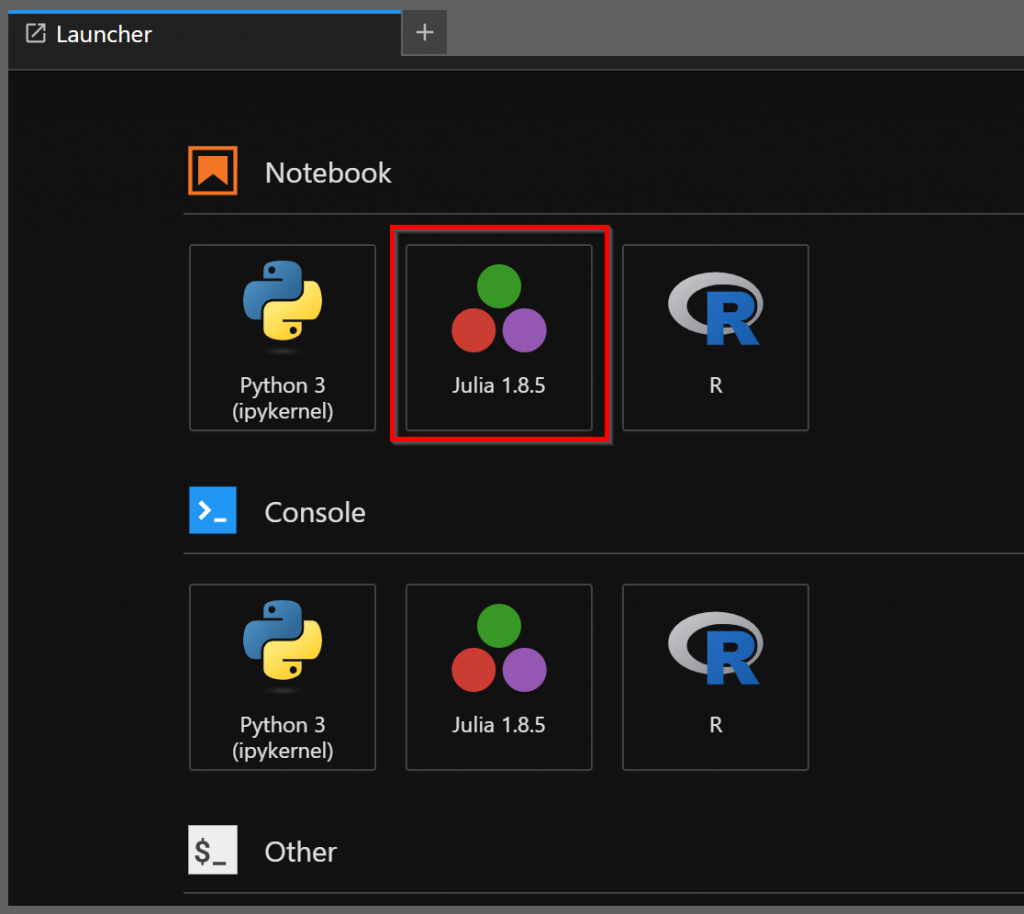
Open a new Jupyter notebook with a Julia kernel.

In the first cell, we are going to make sure we have installed all the packages we need.

import Pkg
Pkg.add("DataFrames")
Pkg.add("Flux")
Pkg.add("MLJ")
Pkg.add("CUDA")
Pkg.add("IterTools")
Pkg.add("ProgressMeter")
Pkg.add("Images")
Pkg.add("Augmentor")
Pkg.add("Glob")
Pkg.add("MLUtils")
Pkg.add("ImageShow")
Pkg.add("Statistics")

Execute this cell and allow it to run. It may take some time, depending on if you have these libraries downloaded and pre-compiled in your environment.

Next, we will import the packages with the Julia using command.

using DataFrames
using Flux
using MLJ
using CUDA
using IterTools: ncycle
using ProgressMeter
using Images
using Glob
using MLUtils
using Augmentor
using CUDA: CuIterator
using ImageShow
using Statistics

Data Preprocessing

Before we start we need to have some data to train and test our network with.

Download the file Churn_Modeling.csv. Copy to a location where you are going to have access to it while programming the neural network. I created a new folder called data and placed the file there.

Import the Data

The first step is to load the data. We are using the Julia package DataFrames.jl. We give the path and the filename and load it to a variable called dataset. Then we take a look at the first 10 rows.

dataset = DataFrame(CSV.File("data/Churn_Modelling.csv"))
first(dataset, 10)

Split the Data into X and y

Next, we are splitting the data columns into X – the feature set – and y – the target values. In the first line, we define an in-line function to detect if the column name does not match one of CustomerId, RowNumber, or Surname. To simplify the data we are training the ANN on, we drop these columns because we don’t think they have information relevant to if the customer stays or leaves the bank.

In the second line, we use the unpack method from the MLJ.jl package. The first parameter is the dataset, the next parameter (==(:Exited)) is a function to determine the columns to go into the first split which is y in our case, the cols function is then provided to match the remainder of the columns for X.

cols(name) = name != (:CustomerId) && name != (:RowNumber) && name != (:Surname)

y, X = unpack(dataset, ==(:Exited), cols)

Encoding Categorical Data

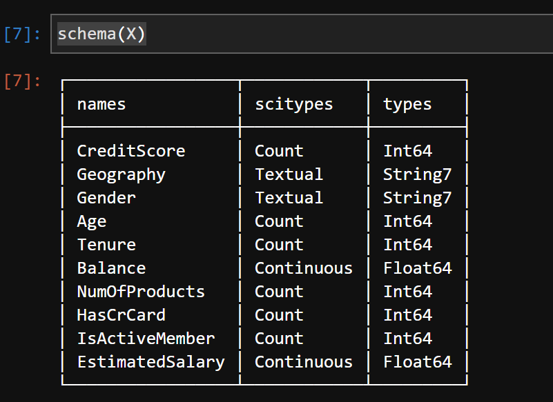
Next, we take a look at the scitypes of the data. More data on these is available here.

schema(X)

One Hot Encode the Gender and Geography Columns

We can see the Geography and Gender are text strings. This isn’t ideal for a artificial neural network, so we want to encode them into numerical values.

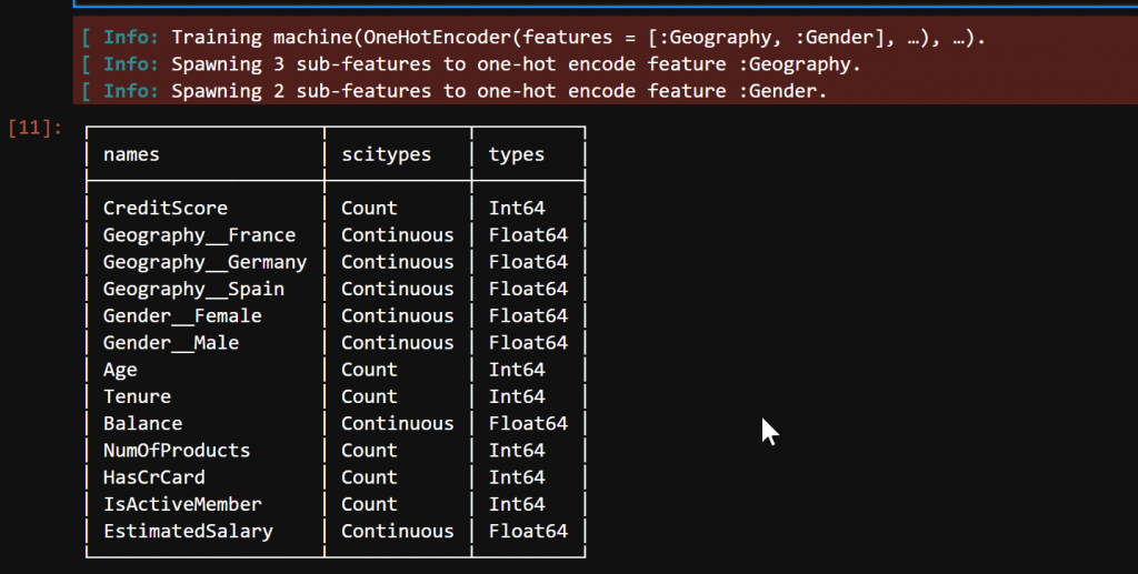
First, we change their scitypes into Multiclass. Then MLJ.jl’s OneHotEncoder encodes the two columns into five columns. Below we see we now have Geography__France, Geography__Germany, Geography__Spain, Gender__Female, and Gender__Male. These are now continuous values. And the original columns have been removed.

X.Gender = coerce(X.Gender, Multiclass)
X.Geography = coerce(X.Geography, Multiclass)

hot_encoder = OneHotEncoder(features=[:Geography, :Gender])
mach = fit!(machine(hot_encoder, X))
X = MLJ.transform(mach, X)
schema(X)

Looking at the first 10 columns we see they have 1.0 or 0.0 values.

first(X, 10)

Coerce the Remaining Datatypes

Now we coerce the datatypes of the expanded values into OrderedFactors. We have used OrderedFactor here because the columns have an intrinsic positive class – true, false, pass, or fail.

X = coerce(X,
    :Geography__France => OrderedFactor,
    :Geography__Germany => OrderedFactor,
    :Geography__Spain => OrderedFactor,
    :Gender__Female => OrderedFactor,
    :Gender__Male => OrderedFactor,
    :HasCrCard => OrderedFactor,
    :IsActiveMember => OrderedFactor)

Feature Scaling

Before we get to building our artificial neural network, we know we need to have normalized or standardized data. To do so we use the MLJ.jl Standardizer class and fit the machine to the entire feature set. We replace the X feature set with the standardized one.

standardizer_model = Standardizer(count=true)
standardizer_machine = machine(standardizer_model, X)
fit!(standardizer_machine)

X = MLJ.transform(standardizer_machine, X)

Split the Data into Train and Test Sets

And before we get into building and training we are going to follow best practices with machine learning and split our data into training and test sets. We use MLJ.jl’s partition function. Unpack works on columns and partition works on rows. We provide the X and y as a tuple, specify 80% of the data goes into the training set, set the seed value with the rng parameter name, and specify the data is going to come into the method as a tuple with multi=true.

Then we unpack the return values into X and y split by train and set sets.

(X_train, X_test), (y_train, y_test) = partition((X, y), 0.8, rng=43, multi=true)

When we do this we end up with a training set of 8000 rows and a test set of 2000 rows.

Build the Artificial Network

With our data massaged into the shape we want, it’s now time to construct the artificial neural network using the Flux.jl framework.

First Layer

We create the first layer using the Dense layer object from Flux.jl. We specify an input of thirteen parameters, which matches the number of columns in our X feature set. We set the output of the layer to six and then specify relu to have a rectified linear unit as our activation function.

layer1 = Dense(13 => 6, relu)

Second Layer

The second layer is nearly the same. We just change the input to the size we output from the first layer. In this layer, we are going from six inputs to six outputs.

layer2 = Dense(6 => 6, relu)

Output Layer

The last layer we build is the output layer. We take the six outputs from the previous layer and output a single value – this is whether the person will leave the bank or not.

output = Dense(6 => 1)

Build the Network

Now, we put the entire artificial network together using Flux.jl’s Chain object and save it as our model.

model = Chain(layer1, layer2, output)

Run the Data Through Before the Training Cycle

First, let’s test it out to make sure it accepts the data and we also get an estimate of how accurate it is without training. Here we get the results and then convert to 1 or 0 based on whether the estimate is > 0.5. We get a result of 42% which is basically what you would expect from randomly choosing 1 or 0.

output1 = model(transpose(Matrix(X_train)))

mean((output1[1, :] .> 0.5) .== y_train)

Training the ANN

It’s time to train our artificial neural network.

Load Into a Loader and Set the Batch Size

First, we create a Flux DataLoader so we can batch up our training set and set it up to shuffle the batches.

loader = Flux.DataLoader((transpose(Matrix(X_train)), y_train), batchsize=32, shuffle=true)

Setup the Optimizer

Next, we create our optimizer. In this case, we will use the Adam optimizer with a learning rate of 0.01.

optimizer = Flux.setup(Flux.Adam(0.01), model)

Setup Loss Function

Next, we create our loss function. Since we are expecting a binary classification, I have chosen to use logitbinarycrossentropy.

loss(m, x, y) = Flux.logitbinarycrossentropy(transpose(m(x)), y)

Training!

Finally on to the actual training. The training isn’t that complicated. We are going to run the data through ten epochs. Most likely this doesn’t take very long, but you may have longer training schedules you will want to train.

To do the actual training, we pass the loss function, the model of the ANN, the loader with the data, and the Adam optimizer. The ! means the model will get updated in place.

number_epochs = 10
@showprogress for epoch in 1:number_epochs
    Flux.train!(loss, model, loader, optimizer)
end

Determine Training Accuracy

Now, let’s see how our model performed.

86% on the training set, that’s not too bad!

output2 = model(transpose(Matrix(X_train)))

mean((output2[1, :] .> 0.5) .== y_train)

Making Predictions

To make sure we haven’t overfitted and can make useful predictions for the bank, let’s look at some data the network hasn’t seen before.

Single Prediction

We are given the assignment to predict if an individual with the below criteria will leave the bank or not.

We create a data frame with the appropriate columns. We make sure we have one hot encoded for the columns that need it. Then we coerce the data and run it through the predefined standardized.

single_data = DataFrame(CreditScore = [600],
    Geography__France = [1],
    Geography__Germany = [0],
    Geography__Spain = [0],
    Gender__Female = [0],
    Gender__Male = [1],
    Age = [40], 
    Tenure = [3], 
    Balance = [60000],
    NumOfProducts = [2],
    HasCrCard = [1],
    IsActiveMember = [1],
    EstimatedSalary = [50000])

single_data = coerce(single_data,
    :Geography__France => OrderedFactor,
    :Geography__Germany => OrderedFactor,
    :Geography__Spain => OrderedFactor,
    :Gender__Female => OrderedFactor,
    :Gender__Male => OrderedFactor,
    :HasCrCard => OrderedFactor,
    :IsActiveMember => OrderedFactor)

standard_data = MLJ.transform(standardizer_machine, single_data)

Now that the data looks the same as the data it was trained on, we can make our single prediction. It says this person won’t leave the bank, which is correct.

single_prediction = model(transpose(Matrix(standard_data))) .> 0.5

Accuracy of Test Set

Now let’s see how well our mode does on the test set we set aside earlier.

Simply, run the data through the model to get the output.

test_output = model(transpose(Matrix(X_test)))

Let’s look at the results in a confusion matrix from MLJ.jl. This seems pretty close to what they got in the course. To remove an error message, we have to coerce the y_test into an OrderedFactor. If you know why let me know.

ConfusionMatrix()(test_output[1, :] .> 0.5, coerce(y_test, OrderedFactor))

Now let us check the results overall for the test set.

85% – it’s right in line with our training set and an excellent result for only a couple of hours of work.

mean((test_output[1, :] .> 0.5) .== y_test)

Summary

In this blog post, we have covered how to create an artificial neural network that gets decent results using Julia, MLJ.jl, and Flux.jl. There are some further steps we could take to improve the accuracy, but those we can leave for another post. If you have any questions or comments please reach out via my contact page, I’ll always accept feedback on my Julia and machine learning journey.