Convolutional Neural Network in Julia

We are back with the second exercise from the course on Udemy called Deep Learning A-Z: Hands on Artificial Neural Networks. In this exercise we are creating a convolutional neural network to categorize images to be cats or dogs. Once again, the exercises in the course are in Python and TensorFlow but I am doing them in Julia and Flux.

If you haven’t seen the first exercise in the series check it out: Artificial Neural Networks in Julia.

A convolutional neural network is one that uses a convolution layer to reduces the dimensionality of the data and to consolidate . I will cover a convolutional network in another post or you can check out the video below from 3blue1brown.

Our Problem

As stated in the intro our problem is to build an cat or dog identifier from an image. Amazingly, this was virtually impossible 8 years ago, but today we can do it in under a 1/2 hour. We have 10,000 images of cats and dogs to train and validate our classifier. I cannot provide the exact same dataset I used as it seems locked in Udemy, but you can find a cats or dogs dataset on Kaggle.

Implementing a Convolutional Neural Network

Prerequisites for the building this is to have Julia installed and Jupyter notebook instance built and running.

Importing Libraries

Open a new Jupyter notebook with a Julia kernel.

In the first cell, download all the packages we need:

import Pkg
Pkg.add("DataFrames")
Pkg.add("Flux")
Pkg.add("CSV")
Pkg.add("MLJ")
Pkg.add("CUDA")
Pkg.add("IterTools")
Pkg.add("ProgressMeter")
Pkg.add("Images")
Pkg.add("Augmentor")
Pkg.add("Glob")
Pkg.add("MLUtils")
Pkg.add("ImageShow")
Pkg.add("Statistics")

Execute the cell and allow it to run. Depending on if you have these packages installed already and compiled, it may take a minute up to 20 minutes to finish.

Next, import the relevant packages into the project with the using command.

using DataFrames
using CSV
using Flux
using MLJ
using CUDA
using IterTools: ncycle
using ProgressMeter
using Images
using Glob
using MLUtils
using Augmentor
using CUDA: CuIterator
using ImageShow
using Statistics

Data Preprocessing

We start with preprocessing our data to get it into the format the neural network will accept for training and testing.

Get the data, either from the course or from Kaggle. I created a new folder called data and a subfolder called catsndogs. There’s subfolder in those for the training_set, test_set, and under those are cats and dogs folders.

Once we have our data situated, let’s take a look at some examples. Here’s a dog.

dog_img_path = "../data/catsndogs/training_set/dogs/dog.1992.jpg"

dog_img = Images.load(dog_img_path)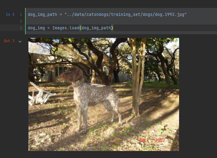

And here’s an image of a cat.

cat_img_path = "../data/catsndogs/training_set/cats/cat.2701.jpg"

cat_img = Images.load(cat_img_path)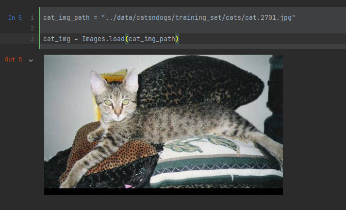

To display them side by side we use mosaicview.

mosaicview(dog_img, cat_img; nrow=1)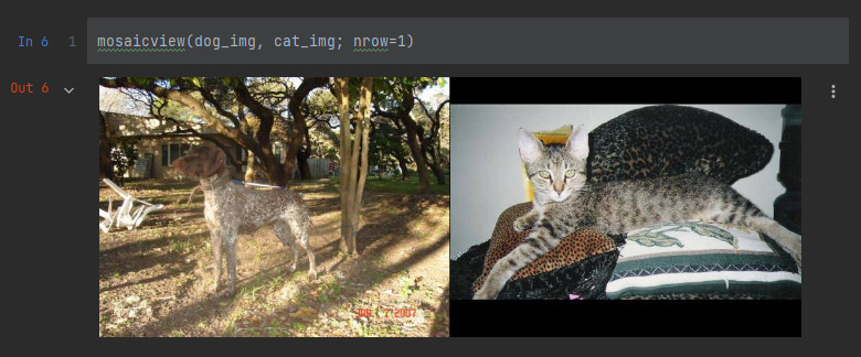

Now let’s look at some of the details of these images.

@show typeof(dog_img)
@show size(dog_img)

@show typeof(cat_img)
@show size(cat_img)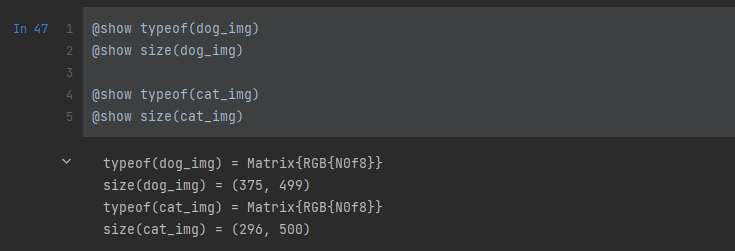

The images are different sizes! Our neural network isn’t going to like that. We will need to resize the images and while we are at it we will do some data augmentation to mix things up a bit.

Let’s set some global variables. We will resize the images to 64x 64 and our neural network will batch them up in groups of 32.

IMAGE_HEIGHT = 64
IMAGE_WIDTH = 64
IMAGE_SIZE = (IMAGE_HEIGHT, IMAGE_WIDTH)
BATCH_SIZE = 32

Importing the Data Sets

Training Set

First we retrieve a list of all the filenames.

training_image_filenames = readdir(glob"*/*.jpg", "../data/catsndogs/training_set/")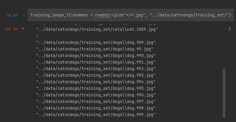

Next, we define our augmentation pipeline to rotate, zoom, flip, and resize the images. In addition, we need to split the images into 3 channels because the Images.jl package in Julia represents all 3 channels in a single layer. Then we change the dimensions because the Images package has the channel as the first dimension and Flux.jl wants the channel as the third dimension. Finally, we we make sure it’s all a Float32.

The load_training_image takes in an image path, loads the image using Image.load, sends it through the augmentation pipeline before returning it.

train_image_transformation_pipeline = 
    Augmentor.Rotate(collect(StepRange(-70, 5, 70))) |> 
    #Augmentor.Zoom(0.8:0.1:1.2) |>
    Augmentor.FlipX(0.5)  |>
    Augmentor.Resize(IMAGE_SIZE...) |>
    Augmentor.SplitChannels() |>
    Augmentor.PermuteDims((3, 2, 1)) |>
    Augmentor.ConvertEltype(Float32)

function load_training_image(image_path)
    image = Images.load(image_path)
    image = augment(image, train_image_transformation_pipeline)
    return image
end

Now we load the training image data. I was able to load all the data into memory, but there are some techniques to only load the data when you need it. I hope to cover that in a future article.

training_image_data = map(filename -> load_training_image(filename), training_image_filenames)

Next, we create the vector of labels by using a map function to determine if the image is in the dogs or cats directory.

training_image_labels = map(filename -> occursin("dogs", String(rsplit(filename, "/")[5])) ? 1.0 : 0.0, training_image_filenames)

Finally, we get to some Flux.jl functionality. We are going to put the data into a DataLoader. Where we allow the data to collate, the batch size is what we defined it above, and the data is shuffled – which we want because we have blocks of cats and then dogs.

training_loader = Flux.DataLoader((training_image_data, training_image_labels), collate=true, batchsize = BATCH_SIZE, shuffle = true)

Now we load the test set using the same steps. Our test set in in a different directory.

test_image_filenames = readdir(glob"*/*.jpg", "../data/catsndogs/test_set/")

We setup our pipeline for the test set. We don’t want to rotate, zoom, or do any augmentation for the test images. But we do need to resize, split the channels, permute the dimensions, and ensure they are all Float32s.

test_image_transformation_pipeline = 
    Augmentor.Resize(IMAGE_SIZE...) |>
    Augmentor.SplitChannels() |>
    Augmentor.PermuteDims((3, 2, 1)) |>
    Augmentor.ConvertEltype(Float32)

function load_test_image(image_path)
    image = Images.load(image_path)
    #image = Images.imresize(image, (64, 64))
    image = augment(image, test_image_transformation_pipeline)
    #image = permutedims(convert(Array{Float32, 3}, channelview(image)), (2, 3, 1))
    return image
end

Next create the data, the labels, and the data loader.

test_image_data = map(filename -> load_training_image(filename), test_image_filenames)
test_image_labels = map(filename -> occursin("dogs", String(rsplit(filename, "/")[5])) ? 1.0 : 0.0, test_image_filenames)
test_loader = Flux.DataLoader((test_image_data, test_image_labels), collate = false, batchsize = BATCH_SIZE, shuffle = true)

Build the CNN

After doing all the preprocessing we are ready to get down to building our model.

Step 1: Convolution

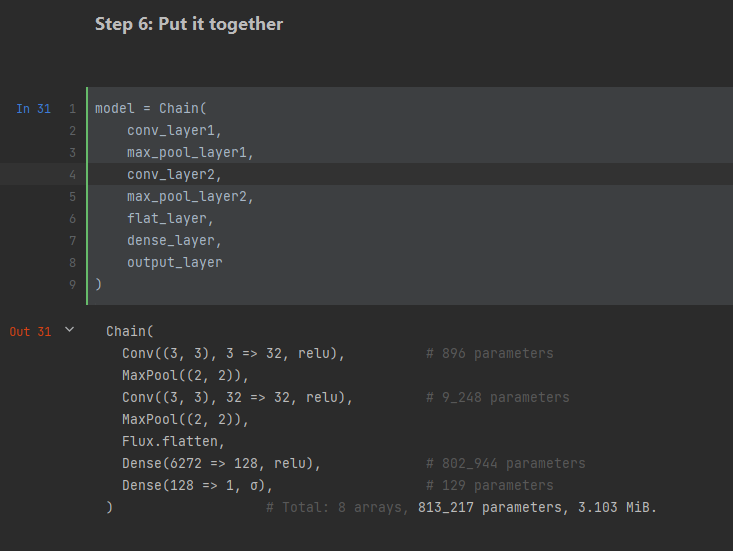
To create the convolution layer we will use the Conv layer from the Flux.jl package. This layer takes in a tuple to define what Flux calls the filter or if you were using TensorFlow, the kernel. The next parameter is a mapping from the number of layers to the outputs of the layer. In our case, the images are RGB with 3 layers and we split it out to 32 outputs. Finally, since this is an internal layer we use relu as the activation function.

conv_layer1 = Flux.Conv((3, 3), 3 => 32, relu)

I like testing out what the layer is going to output, so let’s create a sample dataset and send it through the layer. Our input is the height, width, channels, and batch size, so 64, 64, 3, 32. After running it through the layer we output the size.

xs1 = rand32(64, 64, 3, 32)
conv_layer1(xs1) |> size

Thus the next layer needs to accept an input of (62, 62, 32, 32). The convolution layer will reduce the size of the images.

Step 2: Max Pooling

The next step is to run the data through max pooling. If you want to know more about max pooling either sign up to the Udemy course or check out the below video.

Our max pooling is defined by the MaxPool layer in Flux.

max_pool_layer1 = Flux.MaxPool((2, 2), stride = 2)

Once again, lets test what comes out of this. So we build an array of the size of what came out of our first convolutional layer, run it through the layer, and print out the size.

xs2 = rand32(62, 62, 32, 32)
max_pool_layer1(xs2) |> size

We have reduced the size of our model so it should process faster than if we had left it at 64×64.

Second Layer

We are going to repeat what we did above another convolutional layer and a max pool. Since we have 32 layers now, we will have:

conv_layer2 = Flux.Conv((3, 3), 32 => 32, relu)
max_pool_layer2 = Flux.MaxPool((2, 2), stride = 2)

Testing these two layers together.

xs3 = rand32(31, 31, 32, 32)
max_pool_layer2(conv_layer2(xs3)) |> size

Step 3: Flattening

Next comes the flattening step. This is basically converting the image to a flat row to allow it to go the layer after it. The method in Flux is simply called flatten.

flat_layer = Flux.flatten

And once again, let’s test.

xs4 = rand32(14, 14, 32, 32)
flat_layer(xs4) |> size

As you can see, the flatten layers has turned our image data into one flat vector. The first dimension is the image and the second, the 32, is the batch size.

Step 4: Full Connection

Next, we go back to some standard neural network functionality with a Dense layer. We take the 6272 data points from the flatten, build connections to 128 outputs, and apply a relu activation function.

dense_layer = Flux.Dense(6272 => 128, relu)

Step 5: Output Layer

Our model is finally coming together. We are now constructing the last layer. We have another Dense layer which takes our 128 inputs down to a single output. A single output is all we need because it can be a dog or not a dog (a cat). And since it is the output layer, we apply a sigmoid activation function.

output_layer  = Dense(128 => 1, sigmoid)

Step 6: Put it Together

Now we need to join all these layers together to build our network. To do so we use the Flux.jl Chain object.

model = Chain(
    conv_layer1, 
    max_pool_layer1,
    conv_layer2,
    max_pool_layer2,
    flat_layer, 
    dense_layer,
    output_layer
)

Train the Model

Before we start training we need to establish our optimizer and loss functions. We will use an Adam optimizer and binarycrossentropy for loss.

optimizer = Flux.setup(Flux.Adam(0.001), model)
loss(m, X, y) = Flux.binarycrossentropy(m(X), transpose(y))

Now we are ready to train! We are going to train for 25 epochs and we send it to the Flux.train! method, providing our loss function, the model, the data loader, and the optimizer.

number_epochs = 25

@showprogress for epoch in 1:number_epochs
    Flux.train!(loss, model, training_loader, optimizer) 
end

Testing Single Predictions

Our dataset has some files split out for single testing in a folder called single_prediction. We will see if our classifier can identify these images. We load our images using the load_test_image function. Then display what they are. The displayed images have not been resized.

test_single_image_1_path = "../data/catsndogs/single_prediction/cat_or_dog_1.jpg"
test_single_image_2_path = "../data/catsndogs/single_prediction/cat_or_dog_2.jpg"

test_single_image_1 = load_test_image(test_single_image_1_path)
test_single_image_2 = load_test_image(test_single_image_2_path)
@show size(test_single_image_1)
@show size(test_single_image_2)

img1 = Images.load(test_single_image_1_path)
img2 = Images.load(test_single_image_2_path)
mosaicview(img1, img2; nrow=1)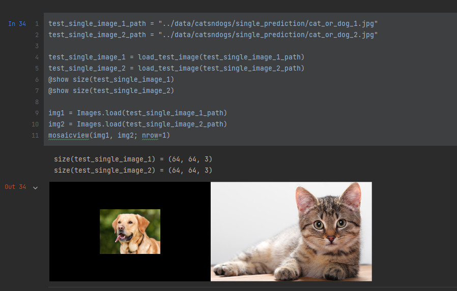

Before we do any testing, let’s convert our outputs into human readable formats with a function called convert_dogcat.

function convert_dogcat(result)
    return map(x ->  x > 0.5 ? "dog" : "cat", result)
end

Now lets see if our model can predict the first image.

single_predict_1 = model(reshape(test_single_image_1, (size(test_single_image_1)..., 1)))
convert_dogcat(single_predict_1)

It was correct, now for the other image.

single_predict_2 = model(reshape(test_single_image_2, (size(test_single_image_2)..., 1)))
convert_dogcat(single_predict_2)

It looks like our neural network is identifying our single test images correctly.

Combine Into A Size 2 Batch

I also want to show how it would look if we combined the two images into a single batch and ran it through our classifier.

So we need to combine these two images into a single batch array. (If you know a better way than this, please let me know!)

batch_array = cat(reshape(test_single_image_1, (size(test_single_image_1)..., 1)), reshape(test_single_image_2, (size(test_single_image_2)..., 1)), dims=4)

And then the batch results show it is processing these images correctly.

batch_results = convert_dogcat(model(batch_array))

Wrapping Up

In this blog post we have gone through the steps to preprocess a set of images, set up a convolutional neural network in Julia, and tested the model on a couple of sample images. For further exploration the reader can attempt to test on the test set and if any one can figure it out, let me know. I tried but failed to figure out how to use the test_loader.